This article is one of a series of tutorials designed to provide the new user with insight into how to create models using the GUI. Advanced users may find the Reference section more helpful.

Introduction to the Experiment Editor

The experiment editor tab is selected using the tab bar on the left side of the GUI window. The image below shows the tab bar (green) with the experiment editor tab selected. You should now select this tab.

Once the tab is selected click the button to ‘Add Experiment’, then click the ‘Done’ button. The experiment editor is now laid out as shown below. The colours highlight the following sections:

Tab selector: This panel is used to change between the different tabs of the GUI. Each tab focuses on a different aspect of model creation.

Component - Create and edit SpineML components.
Network - Create SpineML networks.
Expt - Create and edit experimental procedures for the current model. The current tab is highlighted with a grey background.
Visualisation - OpenGL visualisations of populations and projections for model analysis and the creation of complex connectivity patterns.

Experiment list: This section of the experiment editor tab allows experiments to be added, deleted, selected, and given a name and description. The up and down (^ and v) buttons allow experiments to be re-ordered, the edit button allows the name and description to be changed, and the x button deletes the selected experiment. The RUN button at the top of the panel runs the current experiment using the selected simulator.

expt_overview

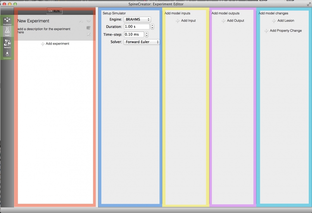
Fig 1: Overview of the experiment editor

Simulator setup: This panel allows the settings for the simulator used to run the model to be configured.

Add model inputs: This panel is used to add inputs into the model.

Add model outputs: This panel is used to log output from the model.

Add model changes: This panel is used to lesion the model by removing Projections, and can also be used to override the values of Parameters and State Variables initial values in the model.

Loading up an example

The following example model will be used to illustrate configuring an experiment: Tutorial model

Download this zip file and unpack it - it contains a folder called Tutorial, inside which is a SpineCreator project file Tutorial.proj.

Setting up the simulator

This panel contains the following settings:

Engine: Select the simulator engine to use. After installation only the default simulator BRAHMS will be available, extra simulators can be added using The ‘Manage simulators’ tab of the Settings dialog (Edit->Settings menu item).
Duration: The duration of the simulation in simulation time. (default 1.0s)
Time-step: The time-step used for the iterative solution of the differential equations. Smaller values lead to more numerically accurate simulations. (default 0.1ms)
Solver: The solution method used to solve the differential equations.

Adding an input

add_input1 add_input2 add_input3

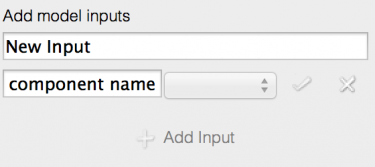
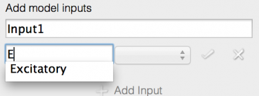
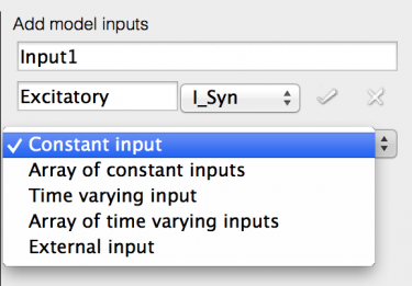
Figs 2-4: Initial input editing

Inputs are added to a model using the ‘Add input’ panel of the experiment editor tab.

Click ‘Add Input’ to add a new input to the model. The new input starts in ‘edit mode’, allowing the input to be configured. The input cannot be added until it is correctly configured.
Rename the input (top text field) to ‘Input1’ as shown.
Click on the text field with ‘component name’ in
Start typing to bring up a list of possible completions from the model - ‘E’ will bring up the Excitatory population.
Note that an incorrect entry will colour the box background red.
Select the Excitatory population.
Now you can select the Port for the input, select ‘I_syn’.

A new drop-down will appear, giving a choice of input types:

Constant input: A single value input to all components in the target for the duration of the simulation. Fields are:
- Value: The value to be input.
Array of constant inputs: A single value to each individual component in the target for the duration of the simulation. Fields are:
- Value: A spreadsheet of all the component indices with one value for each component.
- Fill: This field and button allow the entry of a single value which will be copied to every box in the spreadsheet. Useful if most components take a standard value and only a few differ.
Time varying input: A single value input to all components that can change over the duration of the simulation. Fields are:
- Time: A spreadsheet column containing a time in milliseconds from the start of the simulation for the value to change.
- Value: A spreadsheet column containing the value to change to at the corresponding Time.
- Add row: Adds a new row to the end of the spreadsheet.
- Remove row: Removes the row from the end of the spreadsheet.
Array of time varying input: A single value input to all components that can change over the duration of the simulation. Fields are:
- Selector: The selector to the right of the spreadsheet allows the index of a component to be selected so the Times and Values can be changed for that component. Fields are:
- Time: A spreadsheet column containing a time in milliseconds from the start of the simulation for the value to change.
- Value: A spreadsheet column containing the value to change to at the corresponding Time.
- Add row: Adds a new row to the end of the spreadsheet.
- Remove row: Removes the row from the end of the spreadsheet.
External input: Allows an external source to input values to the model via a TCP/IP connection. The network protocol is described elsewhere on this site. Fields are:
- Command: The path of a command to launch if required to start the source.
- Port: The TCP/IP Port to use to connect (NOTE: do not use in-use ports; 49152 through 65535 are normally safe. The input program you use must be configured to connect on the same port).
- Size: The size of the input source - must be equal to the size of the target of the input (NOTE: This is used for validation and will probably be automated in the future…).

input_ac Fig 5: Constant input

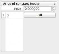input_ac Fig 6: Array of constant inputs

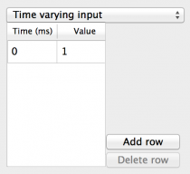input_ac Fig 7: Time varying input

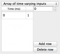input_ac Fig 8: Array of time varying inputs

input_ac Fig 9: External input

Figs 5-9: Input type configuration panels

input_complete

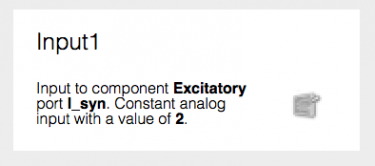
Fig 10: Completed input

The ‘tick’ button confirms the settings for the input, and the ‘cross’ button removes the input.

Choose Constant input, set the value to 2.0, and click the ‘tick’ button to complete the input.

Note that there is now a box with a description of the input and a button to change the input’s settings, as shown in Fig XX.

Adding an output

output_edit

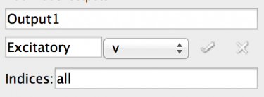
Fig 11: Editing an output

Click ‘Add Output’ to add a new output to the model. The new output starts in ‘edit mode’, allowing the output to be configured. The output cannot be added until it is correctly configured.
Rename the output (top text field) to ‘Output1’ as shown.
Click on the text field with ‘component name’ in
Start typing to bring up a list of possible completions from the model - ‘E’ will bring up the Excitatory population.
Note that an incorrect entry will colour the box background red.
Select the Excitatory population.
Now you can select the Port for the output, select ‘v’ to log the voltage.
Now there is a box for the indices to log. This can be a commas separated list of indices or ‘all’ to log all indices. (NOTE: as of writing BRAHMS does not support limited list and will always log all indices).

output_completed

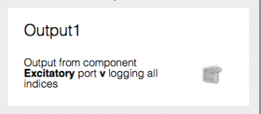
Fig 12: Completed output

The ‘tick’ button confirms the settings for the output, and the ‘cross’ button removes the output.

Click the ‘tick’ button to complete the output.

Note that there is now a box with a description of the output and a button to change the output’s settings, as shown in Fig XX.

Adding a Lesion

Click ‘Add Lesion’ to add a new lesion.
Select the Projection to lesion using the auto-complete field.

Adding a Property Change

Click ‘Add Property Change’
Type the name of the Neuron Postsynapse or WeightUpdate in the auto-complete box.
Select the name of the Property to change from the drop-down menu.
Set the new Property value using the same interface as in the Network editor tab.

Running the experiment

The experiment can be run using the ‘Run experiment’ button at the top of the experiment list.

Visualising the results

We will now look at the methods of visualising the results. First using graphs.

Plot the membrane potential and spikes

Add a new output to the experiment logging the spikes of the Inhibitory population.

Now run the experiment.

If you select the ‘Graphs’ tab you will see that the logs have been added to the ‘Loaded logs’ section.

To add a plot of a log:

Select a clean plot window
Select the log to display
Select the indices to display (ctrl-A (Cmd-A on Mac) selects all)
Choose the plot type (currently only ‘line’ for analog and ‘raster’ for event)
Click the ‘Add plot’ button

You can scale the plot using the mousewheel, drag the plot around, and toggle zooming and dragging on each axis by right clicking on the axis and selecting the menu item.

Deleting graphs is done by selecting them and right clicking to being up the context menu. Select ‘Remove selected graph’ or ‘Remove all graphs’.

The axes can be reset by selecting ‘Scale axes to fit’ from the context menu.

You can add new plots, save plots as PDF or PNG,tile the plots, open data for plotting manually and manually refresh the loaded data using the toolbar items.

COBA_graphs

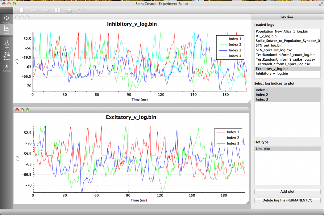
Fig 13: The membrane potentials of the first few neurons of each Population in the COBA example

SpineML The Spiking Neural Mark-up Language