SpineML The Spiking Neural Mark-up Language
Component tutorial
This article is one of a series of tutorials designed to provide the new user with insight into how to create models using the GUI. Advanced users may find the Reference section more helpful. Note that the screenshots are from the Mac build of the GUI, and will have a different visual appearance on other platforms.
Introduction to the Component Editor
 Fig1: Tab selector
The component editor tab is selected using the tab bar on the left side of the GUI window. The Fig 1 shows the tab bar with the Component editor tab selected. You should now select this tab.
Once the tab is selected, the component editor is laid out as in Fig
-
The colours highlight the following sections:
-
Tab selector: This panel is used to change between the different tabs of the GUI. Each tab focuses on a different aspect of model creation.
- Component - Create and edit SpineML components.
- Visualisation - OpenGL visualisations of populations and projections for model analysis and the creation of complex connectivity patterns.
- Network - Create SpineML networks.
- Expt - Create and edit experimental procedures for the current model.
The current tab is highlighted with a grey background.
- Component selector: This section shows the components loaded into the GUI. Prefixes denote the component type, and the bracketed value reports the location of the component. Components can be loaded using the ‘Load components’ button (open folder) and created using the ‘New component’ button (blank sheet). Components can be selected for editing here. The background will be one of four colours:
- Green: Component is valid and the latest version can be used in networks.
- Yellow: The component is valid, but is not stored so networks will use the un-edited version.
- Red: Component has failed validation and cannot be stored unless the issues are corrected. Click ‘Validate for use’ to get a list of issues with the component.
- Blue: Component is currently in use in a network - modifying the component is not advised, but is possible.
Clicking on the divider to the right of this panel will hide and show the panel.
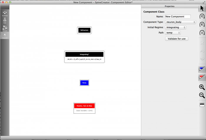
- Component visualisation: This section of the component tab provides an automatically laid out overview of the current component selected for editing. The elements (the building blocks that define behaviour) of the component are displayed visually, and cannot be moved by the user. The display region can be panned by clicking and dragging the background and zoomed using the mousewheel or magnifying glass buttons in the toolbar. The ‘Ports’ and ‘Params, Vars & Alias’ boxes can be hidden or shown using the toggles on the toolbar. Interacting with the component elements will be covered later in this tutorial.
 Fig 2: Overview of the component editor tab
-
Properties panel: This panel is used to edit the properties of the component elements.
-
Toolbar: The toolbar gives context-sensitive buttons for interacting with the current component that is being edited. Note: Hover the mouse over the buttons for a tooltip description.
Example - the LIF neuron and synapse
As an example we will create a Leaky Integrate and Fire (LIF) neuron with a conductance-based single exponential decaying synapse using the component editor tab. The LIF is a simple neuron model that provides a great example for demonstrating the tools. Before getting started building the model we first have a look at the equations that govern the LIF and synaptic model behaviour and show how these should be broken down for implementation.
The equation for the membrane voltage dynamics is:
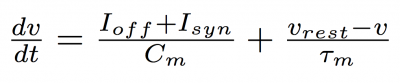
where v is the membrane potential, tau is the membrane time constant, I_off and I_syn are the offset and synaptic currents acting on the membrane, C_m is the membrane capacitance and v_rest is the resting membrane potential.
When the voltage crosses a threshold it is reset to a fixed value and the neuron enters a fixed refractory period in which there are no dynamics for the membrane.
The equation for the synaptic current is:
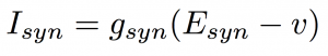
where g_syn is the instantaneous synaptic conductance and E_syn is the synaptic reversal potential.
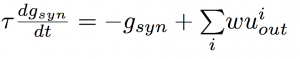
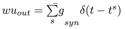
The instantaneous conductance is modelled as follows:
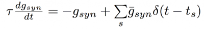
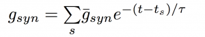
where tau is the synaptic decay constant, s denotes the index in the set of action potential reaching the synapse, and g-bar is the maximal synaptic conductance. The delta function applies an instantaneous rise of g-max to the synaptic conductance each time an action potential acts on the synapse. This equation is more commonly expressed as the solution:
We have tried with the GUI to spare the user as much concern for the implementation of the model as possible to allow them to focus on the model itself, however in mapping these equations to SpineML components we must spare a little bit of thought to implementation.
 showing weight_update (green triangles and postsynapse (red squares)") Fig3: Diagram of a projection between two populations of neuron_body
(blue circles) showing weight_update (green triangles and postsynapse
(red squares)
Fig3: Diagram of a projection between two populations of neuron_body
(blue circles) showing weight_update (green triangles and postsynapse
(red squares)
SpineML has three types of neural components: weight_update, post_synapse, and neuron_body. Together the weight_update and postsynapse components form synapses, however the equations that are placed in each need consideration. Weight_updates are calculated for every connection, while postsynapses are calculated for every target neuron.
The diagram in Fig 3 shows this a bit better - there is a projection between the top population of blue neuron_body components and the bottom blue neuron_body components. Every source neuron_body is connected to every adjacent destination neuron_body. There are seven green weight_updates, but only three red postsynapses - one for each destination neuron_body.
So what does this mean for implementation? Everything that must be done on a per connection basis must be put in the weight_update component, and everything else should go in the postsynapse - as they are fewer in number so will apply less computational overhead. For large densely connected populations unnecessary computation in the weight_update can be quite costly to performance.
For this model this involves breaking the model down as follows:
neuron_body:
postsynapse:
and
weight_update:
where each weight_update i applies each input action potential s for that connection (redefined from earlier), and then the contributions for each weight_update i are summed in the postsynapse. This is possible as exponential decays are linearly separable, so can be composed into a single decay without changing the result.
Sorry about the slight added complexity, but we couldn’t think of a method that would preserve the flexibility and performance we desired and not require this step.
Now that we have the equations that describe the neuron and synapse and have broken them into the correct components, we can begin building!
The IAF neuron_body
Add a new component using the ‘New component’ button at the top of the component selection panel.
First we shall create a SpineML component for the neuron_body. To do that we must add elements to the component and set their properties to create the behaviour we require.
Component properties
 Fig 4: Component properties panel
First we configure the properties of the component as a whole. The properties panel should look as shown to the right (Fig 4). If it does not then make sure the cursor icon is selected in the toolbox and click on the background of the visualisation pane. The properties should be set as follows:
- Name: this is the component name used to reference it. It should be unique and contain no underscroll (_) characters. Set this to ‘IAF’.
- Component Type: leave as neuron_body
- Initial Regime: this cannot be set yet as we have no Regimes
- Path: this is used by the GUI to class components. temp is the default and should be used for components subject to modifications - these must be saved to file before exiting to be preserved. lib is for components to be stored in the GUI’s library, and should be fixed components that you use often. model will be shown if the component has been loaded with the current model. Leave as temp for now.
- Validate for use: this stores the component to memory and checks that it does not contain syntactic errors or omissions. If this is successful the component can be used to build networks.
Add Regimes

Now we add Regimes. These contain sets of differential equations that describe the behaviour of the component in one state.
- Click on the Add Regime button on the toolbox (shown right) to add a Regime.
Regimes: These contain the differential equations that describe the dynamics of the component. Regimes can be switched between using Conditionals (see later). {: .info-popout }
There should now be a new Regime named ‘New_Regime_1’ in the visualisation pane which is selected (note the red outline). In the Properties panel there are the properties that can be set for this Regime, which is just the name. Set the name to ‘Integrating’ - note that the visualisation updates to reflect the changes as you type.
The Add Regime button is no longer on the toolbox as we have the Regime selected, so click on the visualisation pane to deselect the Regime and bring it back. Add another Regime and name it ‘Refractory’.
Click on the background of the visualisation pane to return to the Component Properties and set the ‘Initial Regime’ to ‘Integrating’.
Add a Time Derivative

We now need to add a differential equation element (called a Time Derivatives), which will contain the differential equation for the neuron membrane potential, to the Integrating Regime:
- Select that Regime by clicking on it. The toolbar will now have a new button as shown to the right (Fig 5).
 Fig 5: Time derivative properties panel
- Click this button to add a new Time derivative element to the Regime. The new Time Derivative element will appear with a warning as it is not configured yet.
Select the new Time Derivative element by clicking on it. Note the dotted outline denoting selection of a sub-element. The context sensitive Properties panel now shows the properties of the Time Derivative. The drop down box ‘Variable’ is empty and there are no options to select. We need to add a State Variable for voltage, which will show up here.
Add a State Variable
To add the voltage State Variable:
- First select the red box titled ‘Params, Vars & Alias’ (Note: if the box is out of view click on the visualisation pane and drag to pan the view).
- Note the three new buttons on the toolbar. These buttons allow Parameters (+P), State Variables (+SV) and Aliases (+A) to be added to the system.
State Variables and Parameters: There are two types of Properties of a component - Parameters and State Variables. Parameters represent numbers that are static during the simulation of a model, while State Variables can change, thus they represent the current state of the system. {: .info-popout }
 Fig 6: Right: the toolbar
buttons for adding Parameters, State Variables and Aliases. Left: The
Params, Vars & Alias box
Fig 6: Right: the toolbar
buttons for adding Parameters, State Variables and Aliases. Left: The
Params, Vars & Alias box
- Click to add a State Variable using the centre toolbar button (+SV)
- Select the new State Variable and change the name to ‘v’. The Params, Vars & Alias box should now look like in the above diagram.
- Set the Dimensions to milliVolts by selecting ‘Dimensional Prefix’ of ‘m’ and ‘Dimensional Unit’ of ‘V’.
Finish the Time Derivative
Now we are in a position to finish the Time Derivative we added earlier:
- Select the Time Derivative.
- From the drop-down box for ‘Variable’ select the new ‘v’ State Variable.
- The text in the visulisation pane should update to dv/dt =
Now we add the equation for the membrane potential dynamics. This must be in the form of C-style code (for details see here: section A.1.16 MathInline ). As an example here is the membrane potential equation:
(I_off+I_syn)/C_m+(v_rest-v)/tau_m
where the tau_m has been moved across to the other side of the equation.
Note that there are several names that we use here that represent values that are fixed for the duration of the simulation (I_off, C_m, v_rest, tau_m), or inputs into the component (I_syn), but we have not defined them. Consequently the text background is red - showing that there is an error in the text string. To solve this we must add Parameters for the fixed values, and an Analog Input Port for I_syn.
Your component should now look as below:
Add the Parameters
We now must add the Parameters for the membrane potential equation
To add a Parameter:
-
Select the red box titled ‘Params, Vars & Alias’ as in [[#Add a State Variable adding a State Variable]]. - Click to add a Parameter using the top toolbar button (+P)
Click to add four Parameters, and name these Parameters ‘I_off’, ‘C_m’, ‘v_rest’ and ‘tau_m’.
The Parameters can be re-ordered by selecting one and using the up and down buttons on the toolbar.
Set the Dimensions of the Parameters to physiological units (current = nA, capacitance = pF, voltage = mV, time = ms).
Add the Analog Input Port
Ports: There are three types of Port which carry different types of data between components - Analog Ports carry continuous variable data every timestep of the simulation; Event Ports are analogous to action potential spikes, and trigger discrete events in components; Impulse Ports are event ports that, along with the discrete event, carry a value which can be set by the source component. {: .info-popout }
Ports describe the communications of the component with other components. We need to add an Analog Input Port for the incoming current from the synapses, I_syn.
To add an Analog Port:
- Select the blue box titled ‘Ports’ (Note: if the box is out of view click on the visualisation pane and drag to pan the view).
- Note the three new buttons on the toolbar. These buttons allow Analog Ports (a), Event Ports (e) and Impulse Ports (I) to be added to the system.
- Add an Analog Port, there will be a warning to ‘Select a port variable’ as the port is not configured yet.
- Select the new Port, note the dotted line surrounding it.
The Port is currently configured as an output, or Send port by the ‘Analog Mode’ drop-down box. We want to reconfigure it so that it is an input Port. there are two types of input port: Receive Ports take input from a single source, and connecting multiple sources is not possible; Reduce Ports take input from multiple sources and combine them using a Reduce Operator. Since our neuron may receive currents from multiple synapses, we require a Reduce Port. To configure the Port see Fig 7:
 Fig 7: Reduce Port properties panel
- Change the ‘Analog Mode’ drop-down box to ‘Reduce’
- Set the ‘Name’ to ‘I_syn’
- Leave the ‘Reduce Operation’ as ‘Addition’
- Set the Dimensions to nA
The Properties panel should now look as the image to the right.
Now select the Time Derivative, note that the background to the text is white. If this is not the case then recheck the Parameters and Port for errors.
Add output Ports
We now have a component with membrane dynamics and current input, but we are still lacking any way for the component to communicate to the outside world, and to enter the refractory period. First we consider communication.
The IAF neuron_body needs two outputs. One is an Event Port to transmit spikes, and the other an Analog Port to send voltage for use in a conductance-based synapse.

To add and configure the Analog Port (Fig 8):
- Select the ‘Ports’ box.
- Click the toolbar button to add an Analog Port (a).
- Select the new Port
- Set the ‘Variable’ box in the Properties panel to State Variable ‘v’
This Port will now transmit the value of the voltage State Variable.
 Fig 9: Properties for the Event Port
To add and configure the Event Port (Fig 9):
- Select the ‘Ports’ Box again by clicking its title bar.
- Click the toolbar button to add an Event Port (e).
- Set the ‘Name’ in the Properties Panel to ‘spike’.
This Port will send Events when triggered, but we still need to add a mechanism to trigger this Port.
Introduction to Transitions
In order to move between Regimes, or perform actions within the component that depend upon conditions being met, we use Transitions.
There are three types of Transition:
- OnCondition: This contains a conditional statement, and if this is satisfied then a set of procedures is followed (a traditional if-then statement)
- OnEvent: This is triggered in response to an event on a set Event Port, and contains a set of procedures.
- OnImpulse: This is triggered in response to an impulse on a set Impulse Port, and contains a set of procedures.
For this component we only require OnCondition Transitions. The remaining two Transition types will be described when creating the weight_update component.
All Transition types can contain State Assignments which can update State Variables by assignment - i.e.:
sv1 = sv1+(var1-sv2*exp(var2))
They can also contain EventOut and ImpulseOut which trigger Events and Impulses to be transmitted on set Ports.
Adding an OnCondition for the spike
The three types of Transition are added using the three toolbox buttons below the cursor arrow button (C: OnCondition; E: OnEvent; I: OnImpulse). Clicking these buttons exits the selection mode (denoted by the cursor arrow) and enters a creation mode for the respective Transition. To add an OnCondition Transition (see Fig 10):
 Fig 10: The new OnCondition
- Click to activate OnCondition creation mode (C button).
- Click and drag from the ‘Integrating’ Regime to the ‘Refractory’ Regime - a green arrow shows a valid Transition can be made. Note that Transitions can return to the same Regime they originated from.
- The visualisation pane will update to show the new OnCondition (see right).
Selecting the OnCondition brings three new buttons to the context sensitive toolbar: add State Assignment (=), add EventOut (e^), and add ImpulseOut (I^).
We now need to configure this OnCondition to activate when the neuron reaches a set threshold, then reset the voltage to zero and note the time of the spike (which will be used to return to the ‘Integrating’ Regime after the refractory time period).
Configuring the OnCondition
OnCondition Properties
We now need to apply some of the lessons learned so far to set up the OnCondition, as we need new Parameters for the threshold and reset voltages, a new State Variable to store the spike time, and a new Parameter for the refractory time period:
- Add a Parameter named v_thresh (dims = mV)
- Add a Parameter named v_reset (dims = mV)
- Add a Parameter named t_refrac (dims = ms)
- Add a State Variable named t_spike (dims = ms)
These can then be used to configure the OnCondition:
- Select the OnCondition. The Property ‘Maths’ is the conditional if - set this to:
v > v_thresh
Your component should now look similar to that is Fig 11.
 Fig 11: Overview of the component at this stage
Adding a State Assignment
 Fig 12: State Assignment Properties
We need two State Assignments in this OnCondition. These will reset the voltage to v_reset and log the spike time in t_spike.
- Select the OnCondition by clicking on its title bar.
- Click on the toolbar to add a State Assignment (=).
- Click again to add another.
- Select the first State Assignment.
- Configure as shown to the right (Fig 12).
 Fig 13: ‘t_spike’ State Assignment Properties
We now configure the second State Assignment with ‘Variable’ set to ‘t_spike’. We wish to store the current simulation time, so we use the reserved variable t to do so, setting ‘Maths’ to ‘t’, as shown to the right (Fig 13).
Adding an EventOut
The final thing that the component must do when the voltage threshold is crossed is emit an action potential, or spike. To do this we add an EventOut to the OnCondition.
- Select the OnCondition.
- Click the toolbar button to add an EventOut (e^).
- Select the EventOut and choose ‘spike’ as the Event Port to send the spike on.
Add an OnCondition to return from the Refractory Regime
While in the ‘Refractory’ Regime there are no Time Derivative and the system does not update. We therefore need to add a means of returning to the ‘Integrating’ Regime after the refractory time period has elapsed to allow the component to function again. We do this using another OnCondition Transition.
- Add an OnCondition from the ‘Refractory’ Regime to the ‘Integrating’ Regime.
- Select the OnCondition and set the ‘Maths’ to:
t > t_spike+t_refrac
Now when t has progressed past t_spike by t_refrac (i.e. the current time is the spike time + the refractory time period) the component will transition back into the ‘Integrating’ Regime.
Storing the finished component for use and saving
The component is now complete. However in order to use it in models we must first validate and store the model. To do this:
- Click on the visualisation pane background and click ‘Validate for use’ in the Properties Panel.
or
- In the ‘Component’ menu select ‘Validate component for use’.
To save the model to a file use the ‘Save component’ and ‘Save component as…’ items in the ‘File’ menu. The component will be stored as a SpineML xml file. The model does not have to be stored to be saved, but will be validated before saving.
If there are any validation problems with the model these will be reported and the model will not be stored or saved! Only correctly formed models can be stored or saved
 Fig 14: The finished component
Test the component
We will now quickly run through the steps to test this neuron - note that no explanation will be given here as these are subjects for the remaining tutorials.
- Click on the ‘Network’ tab
- Click ‘Add Population’ from the toolbar (you can find it using the tooltips)
- In the ‘Properties’ pane for the population select ‘Neuron Type’ as your component
- Set the Parameters as follows (Tip - select ‘Fixed’ button for all, then use the tab key to move through them):
- C_m = 1.0
- i_offset = 1.5
- v_thresh = -50
- v_rest = -70
- v_reset = -80
- tau_m = 20
- t_refrac = 5
- And the State Variables to:
- v = -70
- t_spike = 0
- Click on the ‘Expts’ tab
- Click ‘Add experiment’
- Click ‘Add output’
- In the ‘Component name’ box select all and start typing ‘P’ - select ‘Population’
- Select port=’v’ and click the tick button
- Click ‘Run experiment’
- If successful click the ‘Graphs’ tab
- To the right select ‘Population_v_log.bin’, then ‘Index 0’ and ‘Line plot’
- Click ‘Add plot’
You should see regular spiking.
Note: if you play with the parameter and run the experiment again the plot will update with the new results!
The synapse weight_update
It is worth noting that this weight_update component contains no Time Derivatives or Analog Ports. This means that everything in the component acts in response to Events or Impulses - it is Event Driven. By making the weight_update Event Driven the simulation can calculate synapses much faster. You should always aim to make your weight_updates Event Driven for this reason. That said, if it is necessary to add Time Derivatives or Analog Ports then this is possible, however you models will take a significant performance hit for doing so. {: .info-popout }
The synapse weight_update component is simple, but introduces several new component elements - OnEvent Transitions, Impulse Ports and ImpulseOut elements. This section of the tutorial assumes that you have read the previous section.
This component takes a spike from a neuron_body and sends on an Impulse of the connection weight to the postsynapse. It converts an Event into an Event with a value (an Impulse) with the value being the weight of the connection.
Initial setup
- If you have an existing component then select ‘New component’ from the ‘Component’ menu.
- Name the component ‘Static Weight’
- Select a Component Type of ‘weight_update’
- Add a new Regime, Name it ‘default’ and set it as the Initial Regime.
- Add a Parameter named ‘g’ with dimensions nS - nanoSiemens. (Note: this is g_max from the equations, but we call it g here for brevity)
Adding the Event Port
 Fig 15: Event Port properties
We first add the input to the component, which is an Event Port (this will be connected to the Event Send Port of the neuron_body):
- Add a new Event Port and select it
- Change the ‘Event Mode’ to Receive
- Name the port ‘spike’
Currently this event port cannot affect the component behaviour, and requires an OnEvent to trigger when an event is received. First, however, it is useful to add the output port for the component - an Impulse Port.
Adding the Impulse Port
 Fig 16: Impulse Port properties
Now we add an Impulse port that will be the output of the component:
- Select the ‘Ports’ box by clicking its title bar
- Add an Impulse Port using the toolbar button that has appeared (I - hover to check the tooltip if you are not sure you have the right one)
- Select the Impulse Port
- Set the ‘Par/Var’ to ‘g’
- Leave the ‘Impulse mode’ as ‘send’
This configures the Impulse port to send the value ‘g’ when it is triggered - note that g is a Parameter and thus will not change during the simulation as this synapse cannot learn. To implement a learning synapse g would be a State Variable.
Adding an OnEvent Transition
We must now connect the input to the output, which we do using a type of Transition we have not previously used - an OnEvent. The OnEvent is triggered when an Event arrives on the specified Event Port, and can then execute a set of State assignments, EventOuts and ImpulseOuts. We will use the OnEvent to trigger an ImpulseOut and pass on the weight to the postsynapse component.
 Fig 17: OnEvent properties
- Click the button in the toolbar to select ‘Add OnEvent’ mode (E) - use tooltips if you aren’t sure.
- Click and drag within the ‘default’ Regime to add an OnEvent.
- Set the OnEvent Property ‘Event Port’ to ‘spike’
This will be triggered every time the neuron_body connected to the Port ‘spike’ sends an Event.
Adding an ImpulseOut
Now we need to get the OnEvent to send an Impulse.
 Fig 18: ImpulseOut Properties
- Select the OnEvent
- In the toolbar buttons that appear click to add an ImpulseOut (I^) - as always, use tooltips to check the button if you aren’t sure
- Select the new ImpulseOut and set ‘Impulse’ Property to ‘g’.
Now every time the component receives an Event on Port ‘spike’ it will send an Impulse on Port ‘g’. This completes the component! Now validate and store the component and save to hard drive if you wish. Fig 19 shows the finished component.
 Fig 19: Complete weight_update component
The synapse postsynapse
The final component in this tutorial is the exponential decaying postsynapse. This mainly uses the techniques described in the previous sections, so detail will only be provided for the new elements - the Alias and the OnImpulse.
 Fig 20: Postsynapse component after Initial setup
Initial setup
- Name the component ‘Exp decay’
- Set the Component Type to ‘postsynapse’
- Add a Regime named ‘default’ and set as the Initial regime
- Add an Analog Receive Port named ‘v’ (dims = mV)
- Add an Impulse Receive Port named ‘g_in’ (dims = nS)
- Add a Parameter named ‘tau_syn’ (dims = ms)
- Add a Parameter named ‘E’ (dims = mv)
- Add a State Variable ‘g’ (dims = nS)
- Add a Time Derivative to ‘default’ for the equation:
dg/dt = -g/tau_syn
The component should now look like shown to the right (Fig 20).
Note: we have added an input Port g_in, which is not the same name as the output Port g of the weight_update. This is not an issue as the Network Editor will allow differently named Ports to be joined as long as the type and dimensions (if Analog) are consistent, or if Analog one of the Analog Ports has no dimensionality.
Note2: The ‘v’ Port that we have added will need to be connected to the postsynapsic neuron body, this will be covered in the Network Editor tutorial.
Now we will investigate adding an Alias.
Adding an Alias
Aliases are used for two purposes. One is to reduce the length of mathematical expressions by allowing the use of variables which represent a value derived in a separate equation:
dv/dt = I_sum/C_m - v; I_sum = I_off + I_syn + I_noise
Here I_sum is an Alias used to simplify the differential equation.
The second use of Aliases is to derive values for Analog or Impulse Port output. An Analog or Impulse Port may wish to transmit a value derived from the Inputs, Parameters, State Variables and other Aliases of the component. In this case the output I_syn uses the voltage from the neuron_body and the reversal potential (E) to transform the conductance of the synapse into a current.
 Fig 21: Alias Properties
To add the Alias for I_syn:
- Select the Params, Vars & Alias box
- Use the button on the toolbox to add an Alias (+A)
- Select the new Alias
- Set the ‘Name’ Property to ‘I_syn’ and the ‘Maths’ Property to:
g*(E-v)
- Now add an Analog Output Port that transmits I_syn.
Add an OnImpulse Transition
Now the final step in creating this component is to take input from the Impulse Port. To do so we need to use an OnImpulse Transition, the remaining Transition type that we have not used so far.
 Fig 22: State Assignment Properties
To add an OnImpulse:
- Click the button in the toolbar to select ‘Add OnImpulse’ mode (I) - use tooltips if you aren’t sure.
- Select the OnImpulse
- Set the ‘Impulse Port’ Property to ‘g_in’
- Add a State Assignment using the toolbar button (=) and set ‘Variable’ to ‘g’ and ‘Maths’ to:
g+g_in
The component is now finished! validate and store and then save to hard drive if you wish. See Fig 23 for the finished component.
 Fig 23: Finished postsynapse component
Final remarks
I hope this tutorial has introduced you to how to create components in the GUI. Finished versions of the components described here can be found below, and the second tutorial will instruct you how to combine components into networks consisting of neural populations connected by projections. This will also allow you to build networks to test out the components you have just created!
Finished components for reference
Note to selves: ADD FINISHED COMPONENTS HERE