This article is one of a series of tutorials designed to provide the new user with insight into how to create models using the GUI. There is also a SpineML reference page which contains detailed information about the network layer.

Introduction to the Network Editor

The network editor tab is selected using the tab bar on the left side of the GUI window. The image below shows the tab bar (green) with the network editor tab selected. You should now select this tab.

Once the tab is selected, the network editor is laid out as shown below. The colours highlight the following sections:

1. Tab selector: This panel is used to change between the different tabs of the GUI. Each tab focuses on a different aspect of model creation.
   • Component - Create and edit SpineML Component layer items.
   • Network - Create the SpineML Network layer.
   • Expt - Create and edit experimental procedures for the current model. The current tab is highlighted with a grey background.
   • Graphing - Plot graphs of outputs from the model
   • Visualisation - OpenGL visualisations of populations and projections for model analysis and the creation of complex connectivity patterns.
2. Network visualisation: This section of the network editor tab provides a visual overview of the current network. The display region can be panned by clicking and dragging the background and zoomed using the mousewheel. Interacting with and adding objects will be covered later in this tutorial.

Fig 1: Overview of the network editor tab

1. Properties panel: This panel is used to edit the properties of objects.

2. Toolbar: The toolbar gives context-sensitive buttons for adding and removing objects. Note: Hover the mouse over the buttons for a tooltip description.

Example 1 - A Current-Based Vogels-Abbott network

Vogels-Abbott networks provide a good test model for simulators, being both simple and exhibiting of complex yet statistically stable behaviour. Here will will create a single layer Vogels-Abbott network consisting of a population of excitatory neurons and a population of inhibitory neurons with all neurons connected by sparse connection patterns. Here we demonstrate a Vogels-Abbott network using current-based (CUBA) synapses, then one using conductance-based synapses (COBA).

Here are the components needed to complete this tutorial. Use right click to save each XML file. The PNG files show what the component should look like in SpineCreator:

Name	Description	XML	PNG
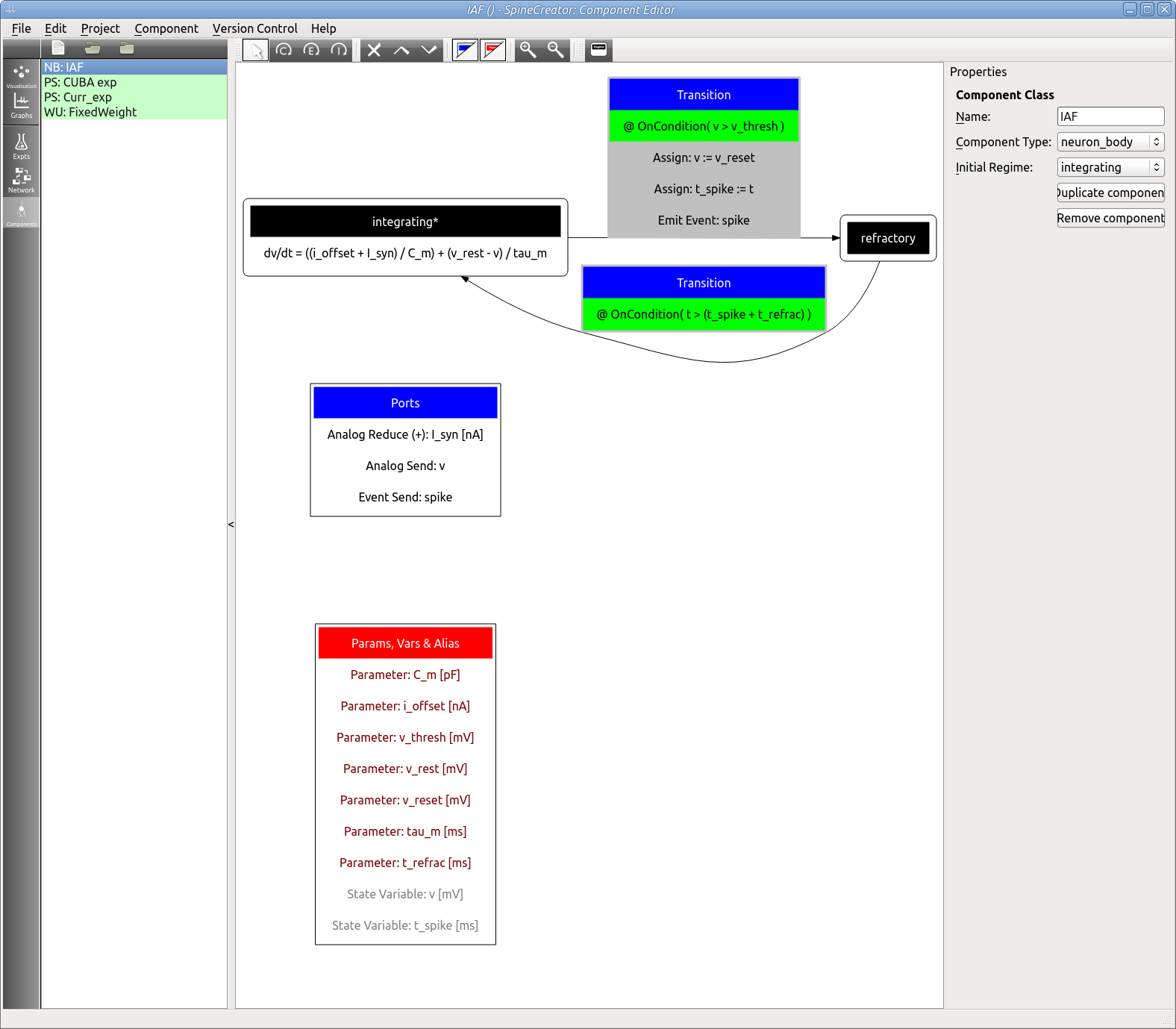
IAF	Leaky Integrate and Fire Neuron Body	IAF.xml	IAF.png
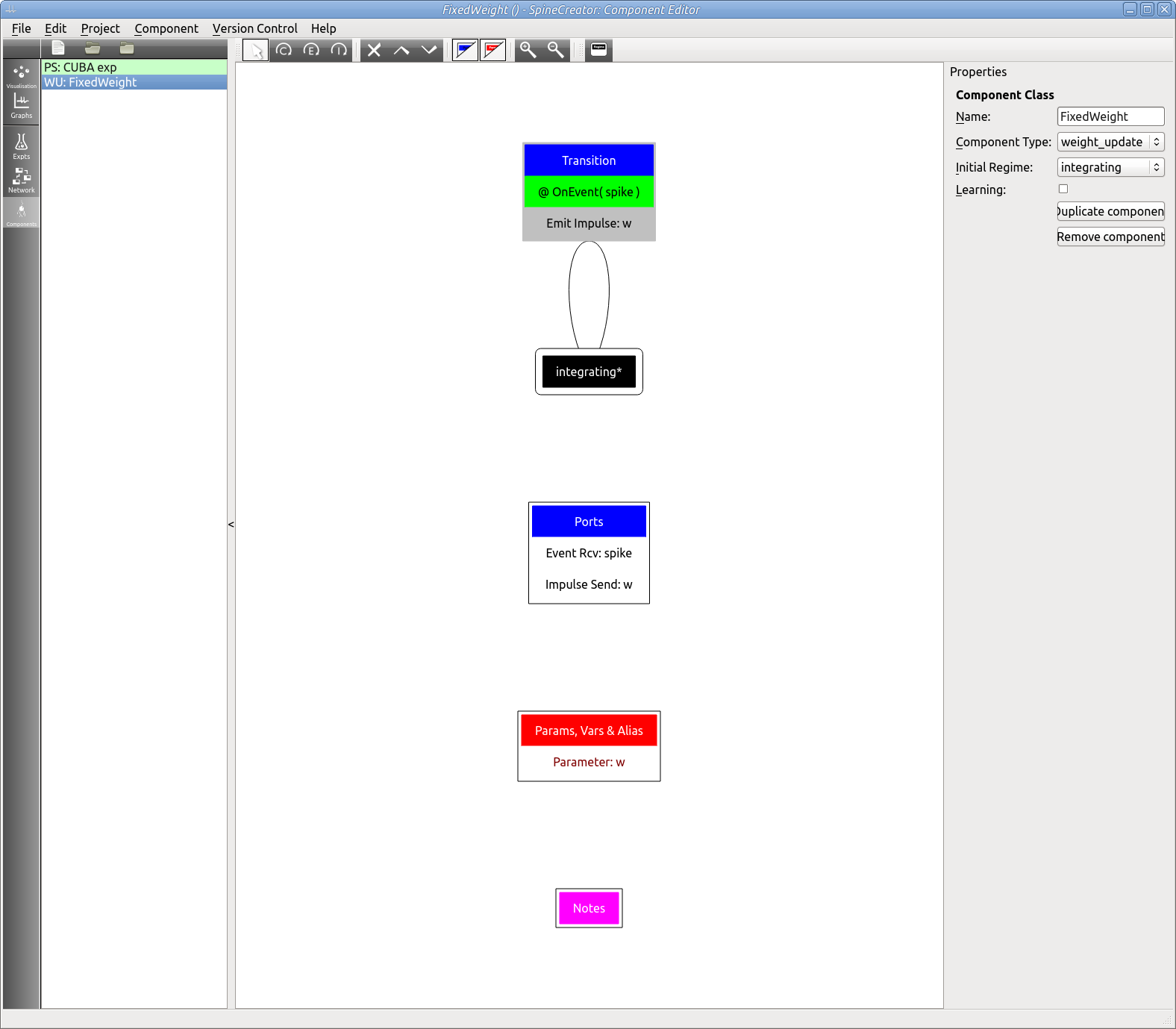
FixedWeight	Fixed Weight Synaptic Update	FixedWeight.xml	FixedWeight.png
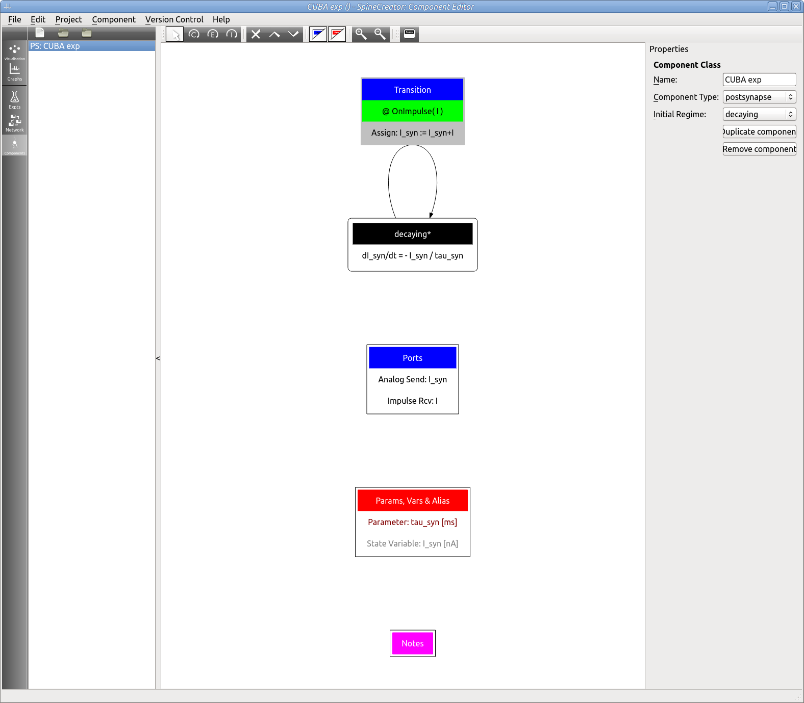
CUBA_exp	Exponentially Decaying Post-Synaptic Current	CUBA_exp.xml	CUBA_exp.png

Introduction to Populations and Projections

IF you have any experience with computational neuroscience then the concept of Populations and Projections will be familiar. It is important, however, to define exactly the properties of these entities within the SpineML framework to avoid any confusion:

• Population: A Population is a set of model neurons of a single type (they all utilise the same neuron_body component). These neurons can have different Parameter values and State Variable initial values, however. In addition, the neurons can be differentiated further by the types of synapse that connect to them. It is possible to connect up one subset of neurons with one type of synapse, and another with a different type, and these two subsets can overlap if required. This can be controlled by the Projections that target the Population.

• Projections: These are synaptic connections between one Population and another with a (currently) fixed connectivity pattern. A projection can contain multiple Synapses each consisting of a connectivity scheme, a weight_update component, and a postsynapse component. The reason for allowing multiple Synapses per Projection is to introduce a clearer way of describing, for example, synapses between two populations that can connect to the apical or basal parts of the dendrite, affecting the neuron differently depending on where they connect.

Creating the populations

We shall first add the Excitatory population of neurons.

Fig 2: Add population

The visualisation pane contains a cursor consisting of a circled cross. This cursor denotes where new populations are added in the visualisation pane’s 2D space. Clicking on a blank part of the pane will move the cursor to that location.

Populations are added using the ‘Add Population’ button on the toolbar (shown right)

• Add a population

Fig 3: Population properties

The new Population is selected and the Properties panel now updates to show the properties of that population. These are:

• Name: Click the ‘Rename’ button and set the population name to ‘Excitatory’. Click the ‘Done’ button to accept.
• Population size: Increase the population size to 3200 neurons.
• Colour: Here the population can be assigned a colour for easier identification. Set the colour to red.
• Neuron tab: This tab allows the selection and configuration of the component that will simulate this population’s neuron. The ‘Neuron type’ drop-down holds a list of all neuron_body type components stored in the GUI. Select the ‘temp/IAF’ component.

The Neuron tab will now contain a list of the Parameters, State Variables and Inputs for this component.

Fig 4: Property selection

Each Parameter of State Variable will have a set of buttons as shown above. These allow the type of value to be set:

• Fixed: All neurons in the population will have the same value, in this case 0.0nA

Fig 5: Fixed value

• Random: All neurons will have a value drawn from a statistical distribution - currently Uniform or Normal. In this case a Uniform distributed value from 0.0 to 4.0.

Fig 6: Random value

• List: All neurons have a unique value. This is set by clicking the ‘Edit’ button and adding values or importing from a comma separated data file.

Fig 7: Explicit values

The x button cancels the current value type choice and allows reselection. Values not set will be assumed to be Fixed Values of 0.0.

For this model we do not require any Lists, and the values should be set as follows:

Fig 8: Values for Excitatory population

Tip: Hold down Ctrl (Cmd on Mac) while moving Populations and Projections to snap them to the grid and create more pleasing layouts!

Now add another Population of neurons:

• Click on the background to set the cursor position.
• Click on the ‘Add Population’ button on the toolbar.

Set up the Inhibitory Population with the same Properties as the Excitatory Population by clicking the ‘Copy’ button on the Excitatory Population Properties and then changing the Inhibitory Population ‘Component type’ to IAF and clicking the ‘Paste’ button. The properties will be as shown below (Fig X):

Fig 9: Configuration for Inhibitory population

Creating the projections

The Vogels-Abbott network is sparsely connected with a fixed probability of connection between any two neurons. To create this we need to add four projections:

Fig 10: An example of a projection with convoluted Beziers!

• Excitatory -> Excitatory
• Excitatory -> Inhibitory
• Inhibitory -> Inhibitory
• Inhibitory -> Excitatory

Adding the projections

Projections are added as follows:

• Select the source Population.
• Click the ‘Add Projection’ button on the toolbar.
• Add intermediate Bezier curves by left-clicking on the background
• Right click to cancel
• Add the Projection by left-clicking on the destination Population.

The Bezier curves can be shaped by clicking on the red ‘handles’ to select and drag them. Selected handles will turn green. Holding Ctrl (Cmd on Mac) will snap the handles to the grid. New Bezier points can be added and removed by right-clicking on the projection line where they are desired.

• Add the four Projections, resulting in a Network similar to below:

Fig 11: The network

Configuring the projections

We now need to configure these Projections. First select the Excitatory -> Excitatory Projection. The properties panel now shows the properties for this Projection:

• Name: Note that this is defined by the names of the source and destination Population names, and cannot be changed. There can only be one Projection between any source and destination population pair.
• Synapse selector: This allows the Projection’s Synapses to be added (+), removed (x) and selected(< and >). The Projection must have at least one Synapse.
• Weight Update tab: Allows the current Synapse weight_update component to be selected and configured.
• PostSynapse tab: Allows the current Synapse postsynapse component to be selected and configured.
• Connectivity tab: Allows the current Synapse connectivity pattern to be selected and configured.

Fig 12: Projection properties

Weight update

Configure as follows:

Fig 13: Configuration for the weight update

Note the Inputs has a entry under it. It you hover the mouse over the name ‘Excitatory to…’ you will get the full text, showing that there is a connection from the Excitatory Population to this Weight Update. The drop-down contains the list of all allowed Port matches (taking dimensionality and data type into account), which in this case is the ‘spike’ output port of the IAF neuron to the ‘spike’ input port of the weight_update. Note: in more complex models this selection may have to be changed.

PostSynapse

Configure as follows:

Fig 14: Configuration for the postsynapse

Connectivity

The Connectivity tab contains a drop-down box for the type of connectivity (default All-to-All), and a Parameter for the delay on the connection. This Parameter can always take a fixed or statistically derived value per connection, and for connections where the number of connections is known in advance it can take an explicit list of values. The types of connectivity are described in full in the reference page.

For this model we need sparse connectivity with a probability of connection between any two neurons of p=0.02. This is created by using a Fixed Probability connectivity with this probability value. We also want a constant 0.1ms delay on all connections.

To configure the connectivity set the properties as follows:

Fig 15: Configuration for the connectivity

Configure the other Projections

The only difference between the remaining Projections and the Excitatory -> Excitatory Projection is the value of ‘w’ for the weight_update component. Configure these as follows:

• Excitatory -> Inhibitory w=0.0162
• Inhibitory -> Inhibitory w=-0.63
• Inhibitory -> Excitatory w=-0.63

Running the network

To run this network, see the tutorial on Creating an experiment.

Saving the network and components

Save the network and the components that make it up using ‘Save project’ from the ‘File’ menu. This will prompt for a path and project file name to save to. Models are saved as a collection of files in a directory in the following format:

• <project_name>.proj This is the main project file and lists the components, network and experiments that make up the spineCreator project
• model.xml This is the network file containing the description of the network.
• experiment.xml These are the experiments (if any) for the model.
• component.xml Other xml files in the directory are the components and are named as per the component name.

Add a new folder using the dialog button and save the model in a new folder named ‘CUBA’.

Fig 16: The save dialog on a Mac - Windows and Linux versions may differ.

Example 2 - Modifying Example 1 to make a Conductance-Based network

Now we have saved the CUBA model we will build on it by modifying the network as a COBA model. This is a simple demonstration of the flexibility of the component-based approach to network building. We will also introduce generic inputs to components, which allow connections between components without using synapses.

Changing the neuron_body properties

The new neuron_body properties are shown below. Note: you can enter the new properties for one neuron_body then copy them to the second.

Fig 17: The properties for the COBA neuron_body

Changing the weight_update

The COBA network using different weights than the CUBA network. In addition we should use a weight_update process that includes the correct dimensions for the weight.

• Switch the ‘Weight Update’ type to FixedWeight.

• Set the weights as follows:

  • Excitatory -> Excitatory g=0.004
  • Excitatory -> Inhibitory g=0.004
  • Inhibitory -> Inhibitory g=0.051
  • Inhibitory -> Excitatory g=0.051

Note that all weights are positive as the sign of the postsynaptic current will be set by the reversal potentials on the postsynapses.

Changing the postsynapse

The COBA postsynapse is the ‘COBA exp’ component. In the ‘Postsynapse’ tab of the projections select this component. Note: the Properties that match between the components are copied across for you.

Now we need to set the reversal potential (E) for each of the projections. The values are as follows:

• Excitatory -> Excitatory E=0
• Excitatory -> Inhibitory E=0
• Inhibitory -> Inhibitory E=-80
• Inhibitory -> Excitatory E=-80

Adding a Generic Input for voltage

Fig 18: COBA voltage port

Fig 19: COBA current alias

Changing the weight_update

The COBA network using different weights than t

The COBA postsynapse is the one created in the Creating a component tutorial. Remember that this component has an input port for voltage that is required to calculate the current (see Fig and Fig). We need now to add a connection that will take the output from the voltage output port of the neuron_body, and input it into the postsynapse ‘v’ port. This is a generic input.

To add a generic input:

• Select the Excitatory to Excitatory Projection.
• Select the ‘Postsynapse’ tab
• At the bottom in the Inputs section there is a box labeled ‘Add from’.
• Begin typing ‘Excitatory’, note the autocompletion
• Select ‘Excitatory’ from the list

Fig 20: Generic input

Fig 20: Generic input visualisation

Note that a new entry appears under Inputs, the port matching has already detected that the only possible connection between these components in the voltage and selected ‘v->v’ as the Ports to connect. Additionally a green loop connects the Population to the Projection.

Configuring the Generic Input

To configure the generic input select it as you would a Projection. Note that like Projections you can add and remove Bezier points using the right mouse button and change Bezier points using the left mouse button.

When selected the Properties panel changes to allow you to edit the generic input’s properties. These are:

• Connectivity This is the connectivity type between the source and destination Ports. One to one is selected and should be left as is.
• Ports The drop-down box allows the valid port combinations to be selected from, as in the component tab of the Projection.

Fig 21: Generic input properties

Now add generic inputs for the remaining Projections.

Add a Spike Input

The aim of the Network Layer / Experiment Layer divide in SpineML is to have a ‘Network as animal’ approach. The Network and Components define an experimental subject and the Experiment is the protocol to be run, including duration, simulation methods, changes to Properties (chemical alterations) and Lesions (physical alterations), outputs (where and what to record from the animal), and inputs (external stimulation to the animal).

It is the final category, inputs, that require further explanation. Inputs can be Analog or Events (including Impulses), with Analog inputs being things like current injection, and Events being spikes. These spikes will arise from brain regions outside the Network, and as such are still part of the animal. For this reason spiking inputs currently require an Object to be added to the Network to act as a conduit, with Projections from this Object channeling the spikes to their targets.

The procedure to add a Spike Source is as follows:

• Click on the Spike Source button on the toolbar (denoted by a spiked line)
• Change the size of the Spike Source to 20
• Connect the Spike Source as in the Figure below.

Fig 22: Spike source properties

Add COBA Synapses to the Excitatory and Inhibitory Populations configured with:

• g=0.1
• tau_syn=5
• E = 0
• Fixed Probability Connection with Probability=0.01 and delay=0

This completes the COBA model, save the model to a new directory named ‘COBA’.

Simulating the networks

The next tutorial will show you how to add an experiment and simulate these Networks.